Training with Image Data Augmentation in Keras

Run in Google Colab

View source on GitHub

Download notebook

In deep learning, we are often limited by the amount of available data and overfitting becomes a real problem. While we could stop the training early or add regularization techniques, it is usually good practice to implement a basic data augmentation in your training routine.

Image data augmentation is very powerful and should be in every deep learning engineer's toolbox!

With good data augmentation, you can start experimenting with convolutional neural networks much earlier because you get away with less data. In Keras, the lightweight tensorflow library, image data augmentation is very easy to include into your training runs and you get a augmented training set in real-time with only a few lines of code.

In this python Colab tutorial you will learn:

• How to train a Keras model using the ImageDataGenerator class
• Prevent overfitting and increase accuracy
• Build a more sample-efficient model

We will also discuss in detail what happened during training and how to spot overfitting.

In the previous posts, we learned about the different data augmentation techniques and how to write your own custom data augmentation preprocessing function. Now it's time to put what we learnt into practice and see what accuracy improvements we get by applying data augmentation!

Setup

We only need a few things to get started, import tensorflow, keras and a few utility functions for label conversion and plotting. Most importantly for this tutorial, we import the ImageDataGenerator class from the Keras image preprocessing module:

import tensorflow as tf
from tensorflow.keras.datasets import cifar10
from tensorflow.keras import layers, models
from tensorflow.keras.preprocessing.image import ImageDataGenerator
from tensorflow.keras.utils import to_categorical
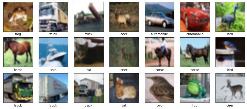
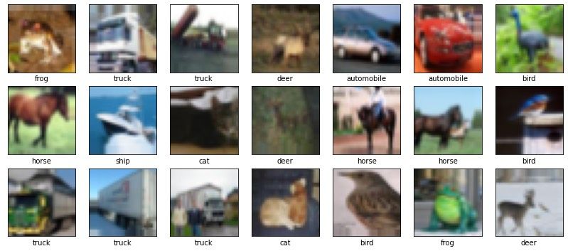
import matplotlib.pyplot as plt

To plot our dataset, we define a visualization function that takes a dataset and simply plots the first few images.

def visualize_data(images, categories, class_names):
    fig = plt.figure(figsize=(14, 6))
    fig.patch.set_facecolor('white')
    for i in range(3 * 7):
        plt.subplot(3, 7, i+1)
        plt.xticks([])
        plt.yticks([])
        plt.imshow(images[i])
        class_index = categories[i].argmax()
        plt.xlabel(class_names[class_index])
    plt.show()

CIFAR-10 Dataset

We are going to build an image classifier. Because the MNIST dataset is a bit overused and too easy, we use the more challenging CIFAR-10 dataset by Alex Krizhevsky, Vinod Nair, and Geoffrey Hinton. It consists of 32x32 pixel images with 10 classes. The data is split into 50k training and 10k test images.

class_names = ['airplane', 'automobile', 'bird', 'cat', 'deer', 'dog', 'frog', 'horse', 'ship', 'truck']
num_classes = len(class_names)

(x_train, y_train), (x_test, y_test) = cifar10.load_data()

x_train = x_train / 255.0
y_train = to_categorical(y_train, num_classes)

x_test = x_test / 255.0
y_test = to_categorical(y_test, num_classes)

visualize_data(x_train, y_train, class_names)

The above code first downloads the dataset. The included preprocessing rescales the images into the range between [0, 1] and converts the label from the class index (integers 0 to 10) to a one-hot encoded categorical vector. Finally we can plot the first few images of the training set.

Classifier Training

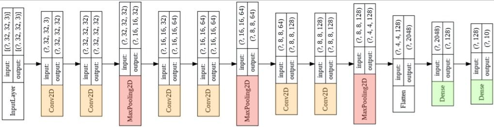
We will use a simple VGG-style convolutional neural network for this model, only a few layers deep. The focus of this tutorial is on data augmentation and we want to train a model in minutes, not hours! Of course if you are interested, you are always encouraged to improve the architecture!

def create_model():
    model = models.Sequential()
    model.add(layers.Conv2D(32, (3, 3), activation='relu', padding='same', input_shape=(32, 32, 3)))
    model.add(layers.Conv2D(32, (3, 3), activation='relu', padding='same'))
    model.add(layers.MaxPool2D((2,2)))

    model.add(layers.Conv2D(64, (3, 3), activation='relu', padding='same',))
    model.add(layers.Conv2D(64, (3, 3), activation='relu', padding='same',))
    model.add(layers.MaxPool2D((2,2)))

    model.add(layers.Conv2D(128, (3, 3), activation='relu', padding='same',))
    model.add(layers.Conv2D(128, (3, 3), activation='relu', padding='same',))
    model.add(layers.MaxPool2D((2,2)))

    model.add(layers.Flatten())
    model.add(layers.Dense(128, activation='relu'))
    model.add(layers.Dense(10, activation='softmax'))

    model.compile(optimizer='adam',
                  loss='categorical_crossentropy',
                  metrics=['accuracy'])

    return model

Below you can see a graphical representation of the model. It consists of three convolutional blocks, each with two convolutional layers, followed by a max-pooling layer. Since we are building a classifier, we flatten the output of the convolutional backbone and add a fully connected inner layer. Finally we add the output layer, which consists of 10 neurons with a softmax activation function.

Train without Data Augmentation

Because our model is so small, we can get away with training it from scratch. We will train it for 16 epochs and use a batch size of 32.
To train the model, we call fit(x_train, y_train), where we pass the training samples and training labels.

batch_size = 32
epochs = 16
m_no_aug = create_model()
m_no_aug.summary()

history_no_aug = m_no_aug.fit(
    x_train, y_train,
    epochs=epochs, batch_size=batch_size,
    validation_data=(x_test, y_test))

loss_no_aug, acc_no_aug = m_no_aug.evaluate(x_test,  y_test)

Note that we keep track of the training history in history_no_aug, which will allow us to compare this training run to the training run with data augmentation in the next step.

Training takes around 11 seconds per epoch on Colab with a GPU, so the whole training run should only take around 3 minutes.

If you follow the output of the training, you already see that this model clearly overfits on the training data!
In my case, the accuracy on the training set was around 94%, while the accuracy on the test set was around 75%.

Training with Data Augmentation

Now let's add data augmentation! We will start by defining our ImageDataGenerator object and specifying the augmentation parameters. For this tutorial, we only use a few parameters:

• width shift: Randomly shift the image left and right by 3 pixels
• height shift: Randomly shift the image up and down by 3 pixels
• horizontal flip: Randomly flip the image horizontally.

When we use that generator in training, the images shown during training will be slightly different every time we feed them to the network. This means that the model will have a much harder time learning features of individual images that are not related to the class. By adding these slight variations, the model will have to learn better features and as a result generalizes better.

For a detailed discussion of the possible augmentation parameters and their effect, see the image data augmentation tutorial.

width_shift = 3/32
height_shift = 3/32
flip = True

datagen = ImageDataGenerator(
    horizontal_flip=flip,
    width_shift_range=width_shift,
    height_shift_range=height_shift,
    )
datagen.fit(x_train)

it = datagen.flow(x_train, y_train, shuffle=False)
batch_images, batch_labels = next(it)
visualize_data(batch_images, batch_labels, class_names)

After defining the the generator, we create a few example images to visualize what is happening in the data augmentation:

For training with augmentation, we can use the same interface we used without augmentation. Instead of passing the training set and training labels, we simply pass the ImageDataGenerator object: fit(datagen). Note that in previous releases of Keras, the function fit_generator() had to be used instead, but now fit() can handle both types of training!

Because we now have a preprocessing pipeline in the training routine, the time per epoch increases considerably: From 11 to 27 seconds.

In terms of overfitting, we are doing much better now! The accuracy on the training set dropped to around 82%, while the accuracy on the test set increased to 80%.

Comparison

Now let's compare the two runs! We write some code to plot the accuracy curves and visualize both training with and without data augmentation:

fig = plt.figure()
fig.patch.set_facecolor('white')

plt.plot(history_aug.history['accuracy'],
         label='train accuracy augmented',
         c='orange', ls='-')
plt.plot(history_aug.history['val_accuracy'],
         label='test accuracy augmented',
         c='orange',ls='--')

plt.plot(history_no_aug.history['accuracy'],
         label='train accuracy',
         c='dodgerblue', ls='-')
plt.plot(history_no_aug.history['val_accuracy'],
         label='test accuracy',
         c='dodgerblue', ls='--')

plt.xlabel('Epoch')
plt.ylabel('Accuracy')
plt.legend(loc='lower right')
plt.show()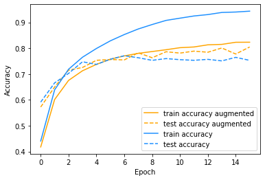

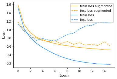
As you can see from the accuracy curve, when training without augmentation, the accuracy on the test set levels off at around 75%, while the accuracy on the training set keeps improving. There is a huge gap between those two curves, which clearly shows that we are overfitting. This can also be seen when you look at how the loss behaves. Without augmentation, the loss on the training set nicely decreases, but the loss on the test set actually increases after epoch 6! Clearly not ideal!

From the accuracy and loss curves, the overfitting is easy to spot!

On the other hand, training with augmentation allows the model to reach a much higher accuracy of about 80%. There is still a difference between the training and test accuracy, so we are probably still overfitting a bit. But it is already much better with only a little bit of data augmentation! Furthermore, you can see that the loss on the test set is still decreasing a bit, so we still have a chance of improving the model by training for longer.

So what is happening here?

When we train without augmentation, we are limited to the images in the training set. These images will be shown to the model over and over again. As a result, the model can start to pick up on specific details in the training data. When we train for long enough, these details will be less and less related to the actual object shown in the image and more related to the background or how the object is placed in the scene. This is clearly not what we want the model to learn.

So therefore, when we vary the image slightly by using augmentation, we make it harder for the model to pick up on these specific features. E.g. when we train with a horizontal flip, we don't destroy any information relevant for the model, but we vary the information that we don't want the model to pick up. This information is for example low-level features at specific locations or the pose of the object we wich to classify.

Conclusion

As you have seen, adding an image data augmentation pipeline when training a model in Keras is super easy and requires only a few lines of code. On our small model, we already saw an increase in the test accuracy of 5%, which is quite significant!

Data augmentation is not only important when the training data is limited, but it can still give a boost in performance even when a lot of data is available.

Data augmentation is one of those techniques that can make or brake an experiment and is a must to master for everyone that trains deep learning models!

As a final note, the Colab notebook is set up so you can explore and experiment! For example, try changing the augmentation parameters and see what happens, or you can try to train the model with only a fraction of the data.

Happy experimenting!