Run in Google Colab

View source on GitHub

Download notebook

Data augmentation is a technique to increase the variation in a dataset by applying transformations to the original data. It is often used when the training data is limited and as a way of preventing overfitting.
Data augmentation is usually done on the fly when training a model. While it can be done, it is usually not practical to store the augmented data on disk. After all, we want to vary the augmented data every time it is shown to the model!

In Keras, there's an easy way to do data augmentation with the class tensorflow.keras.image.preprocessing.ImageDataGenerator. It allows you to specify the augmentation parameters, which we will go over in the next steps. For more details, have a look at the Keras documentation for the ImageDataGenerator class.

Setup

This would be a good point to look at the Colab notebook. You can follow the tutorial by running the code in an ipython notebook on Colab for free, with zero setup! This allows you to play around with the parameters and explore what we discuss here in more detail.
Click the link on the top of the post to either open the notebook in Google Colab or download it to run on your machine.

First we will need some setup code. We start by importing ImageDataGenerator and util functions to load the data.

import numpy as np
import tensorflow as tf
from tensorflow.keras.preprocessing.image import load_img, img_to_array
from tensorflow.keras.preprocessing.image import ImageDataGenerator
import matplotlib.pyplot as plt
import requests

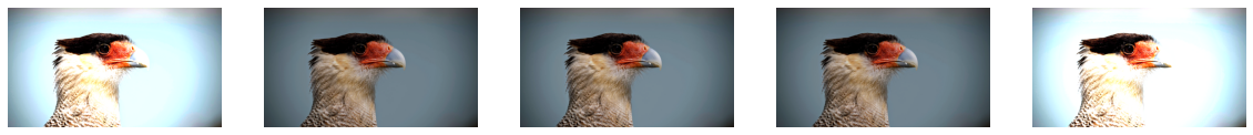
Next we download a sample image from the Github repository, save it locally and load it into memory. And we display the image as a reference of what our input is before data augmentation.

url = 'https://github.com/dufourpascal/stepupai/raw/master/tutorials/data_augmentation/image.jpg'
r = requests.get(url, allow_redirects=True)
open('image.jpg', 'wb').write(r.content)

image = load_img('image.jpg')
image = img_to_array(image).astype(int)
data = np.expand_dims(image, 0)
plt.axis('off')
plt.imshow(data[0])

For ease of use, we define a function that initializes and returns an ImageDataGenerator object that we will then use to set the specific parameters when we visualize the augmentation.
The fil_mode is set to 'nearest' by default, but for the visualizations in this tutorial we set them to a constant black value. You can set different behaviour by specifying fill_mode to one of {'constant', 'nearest', 'reflect', 'wrap'}

def default_datagen():
  datagen = ImageDataGenerator( fill_mode='constant', dtype=int)
  datagen.fit(data)
  return datagen

Next we define a plot function that will take an ImageDataGenerator object and a dataset as input. This function will display a number of augmented images in a grid. Here we see the basic use of the data augmentation pipeline. Calling datagen.flow(data) returns a python generator that returns augmented images. Here we use that generator to get a new augmented image by using next(). We then plot the augmented image and move on to the next one. By default a single row and of five images is plotted, but this can be changed to see more augmented images.

def plot_augmentation(datagen, data, n_rows=1, n_cols=5):
  n_images = n_rows * n_cols
  gen_flow = datagen.flow(data)

  plt.figure(figsize=(n_cols*4, n_rows*3))
  for image_index in range(n_images):
    image = next(gen_flow)
    plt.subplot(n_rows, n_cols, image_index+1)
    plt.axis('off')
    plt.imshow(image[0], vmin=0, vmax=255)

Visualizing Transformations

Now let's visualize the different transformations available in Keras! In each step, we will initialize a default ImageDataGenerator object, then set the augmentation parameters we are interested in, and finally visualize the result.

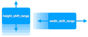
Width and Height Shift

datagen = default_datagen()
datagen.width_shift_range = 0.2
datagen.height_shift_range = 0.2
plot_augmentation(datagen, data)

Shifting an image left and right or up and down can be achieved by using the parameters width_shift_range and height_shift_range.

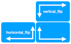
Image Flips

datagen = default_datagen()
datagen.horizontal_flip = True
datagen.vertical_flip = True
plot_augmentation(datagen, data)

Flipping an image horizontally or vertically is achieved by setting horizontal_flip=True or vertical_flip=True. The probability of a flip is 0.5. Keep in mind that vertical flips are often not actually helpful, but this depends on the task. E.g. if we want to identify objects in photos, the objects normally do not occur upside down.

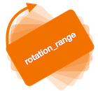
Rotation

datagen = default_datagen()
datagen.rotation_range = 25
plot_augmentation(datagen, data)

A random rotation can be specified in degrees with the parameter rotation_range. The final rotations will be in the range [-rotation_range, +rotation_range].

Zoom

datagen = default_datagen()
datagen.zoom_range = [0.5, 1.5]
plot_augmentation(datagen, data)

zoom_range allows the specification of the random zoom range as a tuple/list of two values [lower, upper]. The value specifies how much the image gets larger or smaller, e.g. a value of 1.0 means no zoom, a value of 0.5 would mean zoomed out so the image is only 50% as large as the input, and a value of 2.0 would mean zoomed in at 200%. Note that the zoom is applied independently on the X-axis and Y-axis! This means that specifying a zoom also leads to stretching.

Shear

datagen = default_datagen()
datagen.shear_range = 20
plot_augmentation(datagen, data)

Shear is a transformation where the image is skewed. Think of it as moving the left edge of the image up, while moving the right edge down (or vice versa). A random rotation can be achieved by specifying shear_range in degrees.

Brightness

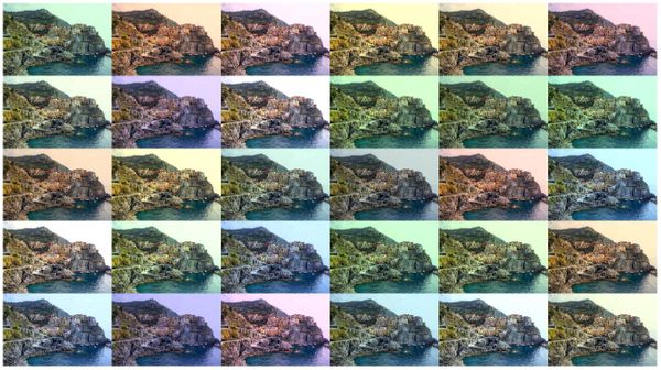
datagen = default_datagen()
datagen.brightness_range = [0.5, 2.0]
plot_augmentation(datagen, data)

The overall brightness of the image can be varied with `brightness_range`.A value of 0.0 is completely black, and a value of 1.0 is the original brightness.A value of 2.0 would mean twice as bright as originally.

Combining Multiple Transformations for Data Augmentation

Now that we understand the individual parameters, let's combine them!
We also specify fill_mode='nearest' to have more naturally looking augmented output images.

In practice, it is always good to look at the output of the data augmentation before you start training. Because we combine multiple transformation, the output images could be deformed too much.

datagen = default_datagen()
datagen.fill_mode='nearest'
datagen.horizontal_flip=True
datagen.width_shift_range=0.2
datagen.height_shift_range=0.2
datagen.zoom_range=[0.8, 1.2]
datagen.rotation_range=20
datagen.shear_range=10
datagen.brightness_range = [0.75, 1.5]
plot_augmentation(datagen, data, n_rows=3, n_cols=5)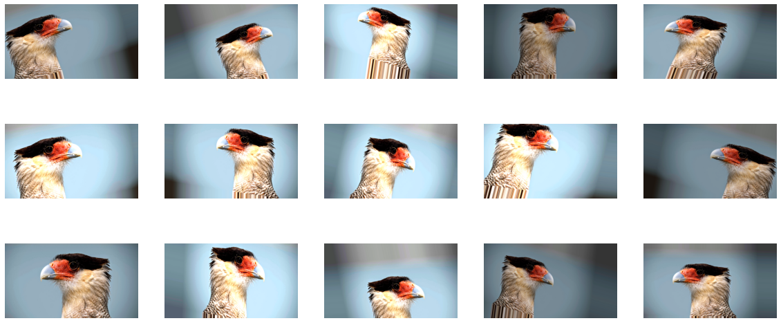

Conclusion

As you can see, we can create an impressive set of variation from just a single sample image. And data augmentation in Keras can be done in a just few lines of code. For standard image classification tasks, this is often sufficent to start and can be used right out of the box.

Next

What I personally would like to see is an option to vary the colors, but this cannot be done out of the box with Keras. For that we have to implement it ourselves: Check out the next tutorial in the series, where we implement our own augmentation transformation!
There is also a post about how to actually train a convolutional neural network with data augmentation.
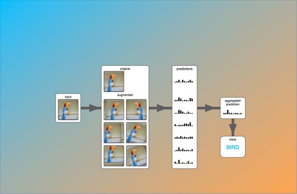
You might also be interested in my test-time data augmentation (TTA) tutorial, where I explain how to properly implement data augmentation for inference to boost a model's prediction accuracy.