How to Correctly Use Test-Time Data Augmentation to Improve Predictions

Test-Time Data Augmentation (short TTA) is a technique that can boost a model's performance by applying augmentation during inference and is a popular strategy to use with deep learning models.
Inference is performed on multiple altered versions of the same image, and
the predictions are then aggregated to get a higher overall accuracy.
Unlike train-time data augmentation, we don't need to make any changes to the model, therefore it can be applied to an already trained model!

Too often have I seen it used in the wrong way, using random data augmentation instead of a set of predefined constant augmentation. The result is a worse performing inference pipeline and unneccessary computations, resulting in a high computational load for inference.

In this post you will learn how to apply test-time augmentation correctly in a production setting and how to find the parameters that work for your model. Read on to learn how to get the most benefit out of your limited inference budget!

The Basics of Test-Time Augmentation

Without test-time data augmentation, inference is very simple: The input image is simply run through the network and we collect the results. Done.
Depending on the type of model, we might have to transform the output of the model to the final format. E.g. in the case of classification, we would usually perform an argmax. The following is an example:

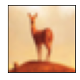
Let's say we have a classifier for CIFAR-10 images that has 10 output classes:
[airplane, automobile, bird, cat, deer, dog, frog, horse, ship, truck]

When we run the above image through a classifier, we get an output like the following:
[[0.08 0.00 0.54 0.01 0.37 0.00 0.00 0.00 0.00 0.00]]
In this case, the image would be wrongly classified as a bird and not as a deer.

To improve this result, we can try to run different versions of the image through the classifier and see what comes out. So let's run the original image and a horizontally flipped image through the network:

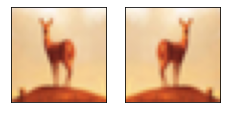
The output of the network will now be two vectors:

[[0.08 0.00 0.54 0.01 0.37 0.00 0.00 0.00 0.00 0.00]
 [0.43 0.00 0.11 0.00 0.39 0.01 0.00 0.01 0.04 0.00]]

The first row is for the original image (same as above) and the second row is for the flipped image. You can see that the model gives the flipped image the highest probability of being an airplane.

When we average the two vectors, we get the vector below:
[[0.25 0.00 0.33 0.01 0.38 0.01 0.00 0.01 0.02 0.00]]
Great! Now the highest probability is given to the class deer.

Now, this image is completely cherry picked and should just serve as an example. In reality, we cannot expect that test-time augmentation solves all our problems. But we can expect that on average we get an improved performance when we use multiple augmented samples instead of just a single input sample!

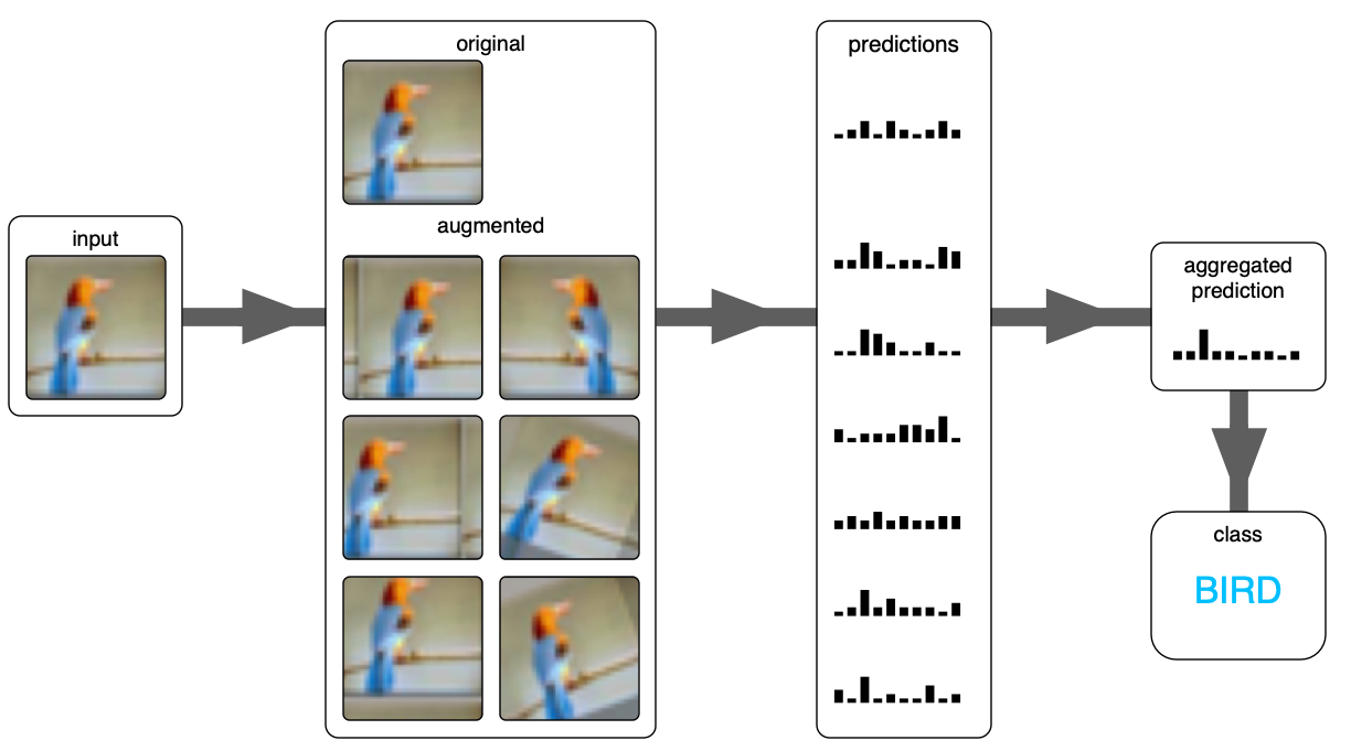
Below is the overall workflow to use with TTA: An input image is augmented, then the augmented and the original image are forwarded through the model, and finally the predictions are aggregated into a final result.

Setup

For this tutorial, we will use transfer learning to very quickly train a simple CIFAR-10 deep learning classifier using tensorflow and Keras. We will then use this classifier to experiment with test-time data augmentation.

Let's start with the inputs. We need just the basics: numpy, tensorflow, Keras, and some utility functions

import numpy as np
import tensorflow as tf
import scipy as sp
from tensorflow.keras.datasets import cifar10
from tensorflow.keras import layers, Model
from tensorflow.keras.preprocessing.image import ImageDataGenerator
from tensorflow.keras.applications import MobileNetV2
from tensorflow.keras.applications.mobilenet_v2 import preprocess_input
from tensorflow.keras.utils import to_categorical
import matplotlib.pyplot as plt
from tqdm import tqdm

We will also define a function to quickly visualize a dataset:

def visualize_data(images, categories=None, class_names=None):
    fig = plt.figure(figsize=(14, 6))
    fig.patch.set_facecolor('white')
    for i in range(min(3 * 7, len(images))):
        plt.subplot(3, 7, i+1)
        plt.xticks([])
        plt.yticks([])
        plt.imshow(images[i])
        if class_names and categories is not None:
            class_index = categories[i].argmax()
            plt.xlabel(class_names[class_index])
    plt.show()

Now it's time to load the CIFAR-10 dataset and visualize the first few images in the test set.

class_names = ['airplane', 'automobile', 'bird', 'cat',
               'deer', 'dog', 'frog', 'horse', 'ship', 'truck']
num_classes = len(class_names)

(x_train, y_train), (x_test, y_test) = cifar10.load_data()
y_train = to_categorical(y_train, num_classes)
y_test = to_categorical(y_test, num_classes)
visualize_data(x_test, y_test, class_names)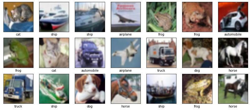

Classifier Training

To speed things up, we will not train a classifier from scratch, but use an existing model trained on imagenet as a feature extractor, and just train a dense layer with those features. The purpose of this tutorial is not to beat the state-of-the-art on CIFAR-10, but rather to have a way of quickly experimenting with test-time augmentation!

def create_model():
    base_model = MobileNetV2(
        include_top=False,
        weights='imagenet',
        pooling='avg',
        alpha=0.35,
        input_shape=(96,96,3),
        )
    base_model.trainable = False

    inputs = layers.Input(shape=(32, 32, 3), dtype= tf.uint8)
    x = tf.cast(inputs, tf.float32)
    x = preprocess_input(x)
    x = layers.UpSampling2D(size=(3,3), interpolation='nearest')(x)

    x = base_model(x)

    x = layers.BatchNormalization()(x)
    x = layers.Dense(128, activation='relu')(x)
    x = layers.Dropout(0.3)(x) 

    outputs = layers.Dense(num_classes, activation='softmax')(x)
    model = Model(inputs, outputs)
    model.compile(optimizer='adam',
                  loss='CategoricalCrossentropy',
                  metrics=['accuracy']
                  )
    return model

As we want a fast model, we use the smallest version of MobileNetV2 as our feature extractor (the base model). We will not train this base model, and therefore set base_model.trainable = False.

On top of the feature extractor we put a batch normalization layer, a small hidden dense layer, and finally the output layer for the 10 classes.

As you can see, the model first upsamples the image from 32x32 to 96x96 pixels. This is because the MobileNetV2 model was trained on imagenet with an input size of 224x224. As a result, the features it computes are somewhat sensitive to the input size and we cannot expect good results if we just feed a tiny 32x32 image as input.

Now it's time to train the model! Because we only train the top, we can get away with just a few epochs:

batch_size = 32
epochs = 5
m = create_model()
m.summary()

history = m.fit(
    x_train, y_train,
    epochs=epochs,
    batch_size=batch_size,
    validation_data=(x_test, y_test),
    verbose=1)

Training the 5 epochs should take less than a minute and in my case the accuracy on the test set reached 0.8097. Now we're ready to start experimenting with test-time augmentation!

How NOT to Do Test-Time Data Augmentation

In the tutorial on training with data augmentation in Keras, we saw that we can use an ImageDataGenerator to generate augmented images on the fly in memroy. This is nice for training, but less usefull during testing.

Wrong: Single Random Augmentation

The code below shows how we should NOT implement a test-time augmentation pipeline.

# accurayc without augmentation
_, acc = m.evaluate(x_test,  y_test)

# augmentation: random flip
datagen_flip = ImageDataGenerator(horizontal_flip=True)
datagen_flip.fit(x_test)

# augmentation: random shift
datagen_shift = ImageDataGenerator(width_shift_range=3. / 32.)
datagen_shift.fit(x_test)

# evaluate once with augmentation
_, acc_flip = m.evaluate(
    datagen_flip.flow(x_test, y_test, shuffle=False)) 
_, acc_shift = m.evaluate(
    datagen_shift.flow(x_test, y_test, shuffle=False))

With the above code, we define two ImageDataGenerator objects, one that randomly flips the image, and one that randomly adds a width-shift to the image. When we then use those to augment the test set, we will not actually use multiple versions of the input image! Each input image is randomly augmented once, and that's it.

Below you see the resulting accuracies with the code below:

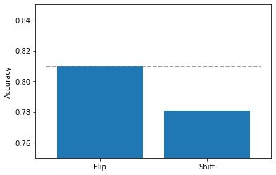
The dotted line represents the accuracy without data augmentation. The two bars represent the results with the two augmentation options we defined. If we perform a random horizontal flip, the accuracy stays roughly the same. This is to be expected because there is no real difference wether the model sees a flipped or non-flipped version of the image. However, for the random width shift, the result is actually about 3% worse! This is most likely because some image information is lost when shifting the original image.

Not Efficient: Multiple Random Augmentations

Ok, but what if we show multiple random augmentations, shouldn't the end result be improved on average?

Well let's try it out! We start by writing an eval_random() function that takes a model and an ImageDataGenerator and dataset as input. First we run the original image without augmentation through the model. Then we run the prediction multiple times with random image augmentations.

def eval_random(model, datagen, x, y, epochs=4):
    datagen.fit(x)

    predictions = []
    acc_history = []

    prediction = model.predict(x)
    predictions.append(prediction)
    for i in range(epochs):
        prediction = model.predict(datagen.flow(x, shuffle=False))
        predictions.append(prediction)

    predictions = np.stack(predictions)
    acc_history = agg_preds(predictions, y)
    return acc_history

As you can see, every time we call model.predict(...) in the loop, a different augmented version of the image will be shown to the model. As a result we get many predictions for many sightly different versions of the original input.

We then also need to write an aggregation function that takes all thos predictions, and outputs a single prediction. Normally we would simply average all the predictions. The function below does go one step further and calculates the accuracies we would get for doing 1, 2, 3, ..., n predictions. With that we see how the accuracies change when showing more augmented samples.

def agg_preds(predictions, y):
    y_classes = np.argmax(y, axis=1)
    acc_hist = []

    for i in range(predictions.shape[0]):
        pred_agg = np.mean(predictions[:i+1], axis=0)
        preds = np.argmax(pred_agg, axis=1)
        acc = preds == y_classes
        acc = np.mean(acc)
        acc_hist.append(acc)
    return acc_hist

We then run the experiment with the following code:

epochs = 16
acc_flip = eval_random(m, datagen_flip, x_test, y_test, epochs=epochs)
acc_shift = eval_random(m, datagen_shift, x_test, y_test, epochs=epochs)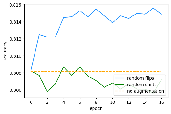

Epoch 0 is the result with only the original image. In epoch 1 we show one augmented image, in epoch 2 we show two, etc.

The result is interesting because the version with random flips improves immediately! What happens is that with two epochs, we probably already have quite a few samples where both the original and the flipped images were shown during inference. The more epochs we repeat this for, the better things become, until we reach a plateau. This plateau is where the original and flipped versions are shown roughly 50-50, so the result becomes balanced.
You might already have notices that a much smarter way would be to show exactly once the original and once the flipped version. And you're absolutely right! Keep on reading to learn the much more efficient way to do TTA in the next section.

For the random shifts, there is no clear benefit of adding more random augmentations. The negative effect of destroying information outweighs the benefit of the augmentation.

Efficient Test-Time Augmentation for Production

As you have seen above, there is really no point in using random data augmentation during inference. Remember, we want to show as few images as possible to keep the inference time low! E.g. if we run the inference on the original image and on a flipped version of it, we already double our inference time!
Therefore, a much better strategy is to use only a few augmented images with predefined augmentation parameters. Also very important is to always show the original image alongside the augmented versions.

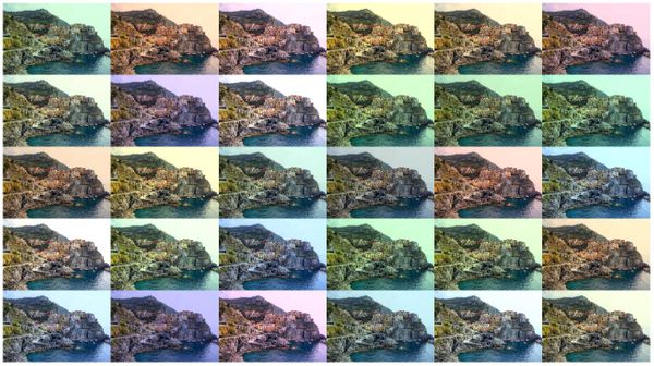
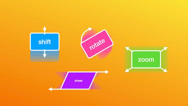
We start of by defining a few functions to flip, shift and rotate a whole dataset. Each function takes a dataset (multiple images) together with an augmentation parameter, and returns a new altered dataset of the same shape.

def flip_lr(images):
    return np.flip(images, axis=2)

def shift(images, shift, axis):
    return np.roll(images, shift, axis=axis)

def rotate(images, angle):
    return sp.ndimage.rotate(
        images, angle, axes=(1,2),
        reshape=False, mode='nearest')

We can then create the augmentations we need as follows:

pred = m.predict(x_test)

pred_f = m.predict(flip_lr(x_test))

pred_w0 = m.predict(shift(x_test, -3, axis=2))
pred_w1 = m.predict(shift(x_test, 3, axis=2))

pred_h0 = m.predict(shift(x_test, -3, axis=1))
pred_h1 = m.predict(shift(x_test, 3, axis=1))

pred_r0 = m.predict(rotate(x_test, -10))
pred_r1 = m.predict(rotate(x_test, 10))

In the above example, we create predictions for the original test images, the flipped images, the width- and height-shifted images, and rotated images.

We then define an aggregation function that takes a set of predictions, averages them, and calculates the final accuracy.

def agg_acc(predictions, y):
    y_classes = np.argmax(y, axis=1)
    pred_agg = np.mean(predictions, axis=0)
    preds = np.argmax(pred_agg, axis=1)
    acc = np.mean(preds == y_classes)
    return acc

Now we can start to experiment with different combinations and see what type of image data augmentation leads to a good model performance.

preds_f = np.stack((pred, pred_f))
acc_f = agg_acc(preds_f, y_test)

preds_w = np.stack((pred, pred_w0, pred_w1))
acc_w = agg_acc(preds_w, y_test)

preds_h = np.stack((pred, pred_h0, pred_h1))
acc_h = agg_acc(preds_h, y_test)

preds_hw = np.stack((pred, pred_h0, pred_h1, pred_w0, pred_w1))
acc_hw = agg_acc(preds_hw, y_test)

preds_fhw = np.stack((pred, pred_h0, pred_h1, pred_w0, pred_w1, pred_f))
acc_fhw = agg_acc(preds_fhw, y_test)

preds_r = np.stack((pred, pred_r0, pred_r1))
acc_r = agg_acc(preds_r, y_test)

preds_fhwr = np.stack((pred, pred_h0, pred_h1, pred_w0, pred_w1, pred_f, pred_r0, pred_r1))
acc_fhwr = agg_acc(preds_fhwr, y_test)

Remember that when we run the code above, we already have the predictions from the classifier. In the code above we simply aggregate the predictions to check what combinations lead to a good result.

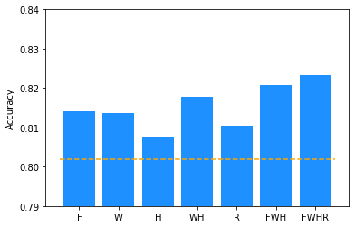
Variable Name	Augmentation	N images	Accuracy
acc	none	1	0.8020
acc_f	flip	2	0.8140
acc_w	width-shift	3	0.8136
acc_h	height-shift	3	0.8077
acc_hw	height-shift & width-shift	5	0.8178
acc_fhw	flip & height-shift & width-shift	6	0.8208
acc_r	rotation	3	0.8105
acc_fhwr	rotation & flip & height-shift & width-shift	8	0.8232

The table above shows the results of running the inference with augmentations. We have an accuracy of 0.802 without augmentation. When we also use a flipped image, we double the inference time, but reach an accuracy of 0.814.
Shifting the width reaches a similar accuracy as with the flip, but we have to do three inference runs. A combination of flip, width- and height-shift leads to a roughly 2% higher accuracy, but the inference will take 6 times longer. Using all of our augmentations (rotation, flip and shifts), we reach an accuracy of 0.8232. Not bad, that's an error reduction of over 10 percentage points!

Best Practices for Test-Time Augmentation

In the next section you will find practical tips and tricks for applying test-time augmentation in production.

Know Your Inference Budget!

First and foremost, you need to know how much time can be spent during inference. If you need real-time predictions, test-time augmentation might not be an option. But in many cases, it might be feasible to spend a bit more time to get a higher performence in return.

First fix the number of augmented images processed in production to fit your requirements, then run experiments to find the best combination of augmentations.

After you optimize a model for production (with a specific optimized inference library or quantization for example), you should know how much time you can spend. Do you have time to process just two images? Then you might want to try using a flipped image in addition to the original one. Or if can you process 4 version of the image? Then run some experiment to find the best 3 augmentation parameters to use.

Note that this comes after you trained and optimized your model!
I suggest first fixing your inference budget because this will give you a clear optimization goal.

Finding the Best Augmentation Parameters for TTA

Once you have your inference budget, it's time to find the best combination of augmentations. This is very similar to hyperparameter optimization during training. There are automatic tools to do this, or you can perform a grid search.

1. Optimize augmentation parameters sparately: I would suggest you start by optimizing on only one augmentation parameter. E.g. find the best width- and height-shift parameters, the best rotation angle, etc.
2. Find the best combination of N augmented images: From step 1, you should know what parameters work well. Now you can try to combine multiple augmented images to get the best result. E.g. you might use a flipped image, and a shifted image. In this step you still don't combine multiple parameters into a single augmentation.
3. Combine multiple augmentation parameters: As a last step, you can try to combine multiple parameters for a single augmentation. E.g. you might try to the original and a flipped image, and a shift on the original and the flipped image.

The whole process is very iterative and probably requires some support code, e.g. to run an automatic search on one or multiple parameters. But because we're only doing inference, the processing time is quite low, so it shouldn't take a lot of time.

Note that these experiments should be done on the validation and not on the final test set! You don't want to optimize towards your test set!

Test-Time Augmentation vs Ensemble Methods

You might wonder how test-time augmentation compares to using an ensemble of models. In general the two methods are quite similar. TTA can be seen as a data ensemble method. There is no generic anser to what method is better and it will depend on your use case. I would suggest testing both methods to measure what performance you get from either one.

However, there are some implications when running in production! Using TTA requires only one model and a small augmentation preprocessing pipeline. On the other hand, running an ensemble of models might be more difficult in production, e.g. when you have to deploy the different models to different GPUs due to memory constraints.

Test-Time Augmentation for Object Detection

Object detection also benefits from TTA, with flips and multiple input resolutions being the most commonly applied augmentation techniques.

The reason for using multiple scales in the inputis that the object detector might be more sensitive towards specific sizes of the objects in the image. E.g. a face detector might have been trained on specific image sizes and might have seen a lot of faces a particular size. As a result, it might be very good at detecting faces in these size ranges, but might not perform very well on much smaller faces. When you then run a higher resolution image through the model, you give the model a chance to also detect those smaller faces.

Merging the detections of augmented images is challenging and because you need to dis-augment the model's predictions.

In object detection, you cannot simply average the final result (e.g. the bounding boxes), but need to aggregate the output of the model. In practice this means that you have to first dis-augmente the model's output (e.g. down-sample the model's output if you used an up-sampled image as input). Then you aggregate the predictions, and finally you perform the non-maxima-supression (NMS) with the predictions from all inputs.

A good starting point to understand how to perform TTA in object detection is RetinaFace and you can check the implementation on their github repository.

Test-Time Augmentation for Image Segmentation

Similar to object detection, TTA also works well in image segmentation tasks. Ayhan and Berens used crops, color transformations and flips in the task of fundus image segmentation. They note that in addition to higher accuracy, the uncertainty estimation becomes more stable when using this test-time augmentation pipeline.

Moshkov et al. evaluated TTA on fluorescent microscopy image and histopathology segmentation. They show a statistical significant improvement when using augmentation in their testing pipeline. The evaluated architectures were U-Net and Mask-RCNN. The use of Mask-RCNN is interesting because the final aggregation step is non-trivial, since Mask-RCNN is instance aware. Check their publication for more details.

Conclusion

While test-time data augmentation is not a magic bullet, it can reduce the error of a model significantly! And the best thing is that it does can be applied post-training and does not require any changes to the model.

As we have seen, it is important to understand the trade-off between inference time and accuracy gain. While random TTA could work well in an academic setting without limitations of processing time, it is not suitable in a production environment.

If you made it this far, you should have a good understanding of how to optimize your model's performace using only a few specific image augmentations. Plus by now you know how to find those augmentation parameters by first fixing the inference budget and then performing a parameter search.